The current trend in AI research is to create very large models trained on massive amounts of training data. Such models effectively solve many optimizations, classification, and generation problems, but they also have disadvantages - huge computation resources and energy consumption during training and tuning. Also, they have an extremely large storage size. And all these factors complicate further developers' adoption, making this industry more privatized.
The known solution and the way to reduce model size is pruning. Pruning is the process of removing weight connections or nodes in a network to increase inference speed and decrease model storage size.
There can be different strategies, but the simplest one is to remove weak links. In this work, we're going to describe a simple and automatic pruning strategy using the well-known genetic algorithm (GA) network.
The genetic algorithm (GA) is a method for solving optimization problems based on a natural selection process that mimics biological evolution. This algorithm reflects the process of natural selection, where the fittest individuals are selected for reproduction in order to produce offspring of the next generation.
The genetic algorithm frees the researcher from the problem of choosing the initial network architecture. Making pruning the part of GA, this algorithm also can free the researcher from the problem of choosing a pruning strategy, making the final network architecture highly optimal.
GA Network
For now, let build the initial GA network. The general components of such a network are as follows:
- Gene - the basic block of network, represents a node with some function performed over inputs. When the node is neuron, the function is some activation function like sigmoid or ReLU.
A gene text representation format is
GeneId FnId -< input1_GeneId weight -< input2_GeneId
weight

example:
5 1 -< 1 -1.1361804 -< 2 1.275428- Link - the weighted connection between nodes.
- Genome - represents the entire network with nodes and their connections.
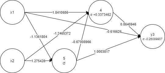
Example genome (the list of genes, textual form of the network graph):
x1, x2, 5 1 -< 1 -1.1361804 -< 2 1.275428, 4 1 0.3373462
-< 1 1.8410686 -< 2 -1.2465372 -< 5 -0.67008966, y3 1
-0.26089907 -< 1 -0.616626 -< 4 0.8640946 -< 5 1.0003817
The same genome formula:

The same genome graph visualization:
- Individual - represents a virtual organism with genome and corresponding fitness.
Fitness is the value of calculating the fitness function with corresponding genome. The fitness function is a single metric objective function used to measure a network quality. - Population - represents an evolving set of individuals.
We've omitted details of implementation, such as species, mutations, environment, and methods, as they are not the subject.
Let start with the simplest example - the XOR classification. Let define our training
environment as:
struct XORClassification;
impl Environment for XORClassification {
fn test(&self, individual: &mut Individual, functions:
&Functions) -> f32 {
let mut output;
let mut distance: f32;
output = individual
.genome
.evaluate(vec![0.0, 0.0], functions)
.unwrap();
distance = (0.0 - output[0]).powi(2);
output = individual
.genome
.evaluate(vec![0.0, 1.0], functions)
.unwrap();
distance += (1.0 - output[0]).powi(2);
output = individual
.genome
.evaluate(vec![1.0, 0.0], functions)
.unwrap();
distance += (1.0 - output[0]).powi(2);
output = individual
.genome
.evaluate(vec![1.0, 1.0], functions)
.unwrap();
distance += (0.0 - output[0]).powi(2);
let fitness = 1.0 / (1.0 + distance);
fitness
}
fn train(&self, individual: &mut Individual, functions:
&Functions) {
individual.genome.train(
vec![
(vec![0.0, 0.0], vec![0.0]),
(vec![0.0, 1.0], vec![1.0]),
(vec![1.0, 0.0], vec![1.0]),
(vec![1.0, 1.0], vec![0.0]),
],
functions,
);
}
fn dropout_condition(&self, fitness: f32, _: f32) -> bool {
fitness >= 0.9
}
fn stop_condition(
&self,
fitness: f32,
complexity: f32,
epoch: usize,
epochs_without_improvements: usize,
) -> bool {
epoch >= 2000 || fitness >= 0.9 &&
epochs_without_improvements > 11
}
}
Here the "test" function calculates fitness, the "train" function provides samples, and the "stop_condition" signals when to stop the evolution. The network evolves by mutating individuals genomes. On each round (epoch), individuals with higher fitness are selected for the next round, and the rest are dropped.
The offspring is generated by mutating selected individuals, and the process continues. The mutation is performed by randomly selecting a mutation from the table, where each mutation has its own probability:
| Function | Probability |
|---|---|
| change link weight | 10 |
| slide link weight | 50 |
| add link | 10 |
| inject gene | 10 |
| toggle function | 10 |
| change parameters | 10 |
From here and below, the node function is Leaky ReLU (all nodes are neurons).
Evaluation result:
epochs=308, time=1.64s, epochs/s=187.8, champion fitness=0.9999999,
genes: 14, links: 35, species=24
x1, x2, 4 1 -< 1 -0.85755104 -< 2 1.083863, 8 1 -0.9924427 -< 1
0.71156317, 11 1 -< 4 0.3792749 -< 8 0.96602243, 15 1 -< 8
-0.6236411, 16 1 -< 15, 9 1 -0.9596125 -< 8 0.47860864 -< 11
1.1306086 -< 15 -0.6067647 -< 16 0.9586857, 13 1 -< 9 -0.7267736,
14 1 -< 9
0.9767301 -< 15 1.0474305, 12 1 -< 16 0.9104208 -< 13 -0.816073, 7
1 -< 12 1.122872 -< 4 1.5250834, 10 1 -< 4 0.63422364 -< 12, 6
1 -< 1 0.8371405 -< 14 0.8477382 -< 10 1.0184075 -< 12 1.0638788, 5
1 -< 2 -0.5893182 -< 4 -0.8171832 -< 6 1.0631118 -< 12, y3 1
0.03961122 -< 2 -0.66733724 -< 5 1.0924925 -< 7 1.007187 -< 8
2.5004368 -< 9 1.1798674 -< 14 -< 15 -0.513005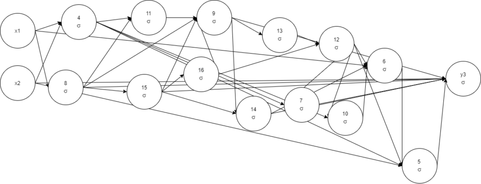
Destructive mutation
As you can see, our network can evolve by tuning weights and growth only. Let extend our mutation table with destructive mutations like unlink and node removal:
| Function | Probability |
|---|---|
| change link weight | 10 |
| slide link weight | 50 |
| add link | 10 |
| inject gene | 10 |
| toggle function | 10 |
| change parameters | 10 |
| unlink | 10 |
| remove gene | 10 |
Evaluation result:
epochs=159, time=627.61ms, epochs/s=253.6, champion
fitness=0.9999999, genes: 4, links: 10, species=33
x1, x2, 5 1 -< 1 0.99010015 -< 2 -0.968485, 7 1 -0.4989009 -< 2
0.17253804 -< 5 0.5081494, 4 1 0.085887074 -< 1 -0.989467 -< 2
0.95624775 -< 7 1.2370766, y3 1 -0.08324337 -< 4 1.0545504 -< 5
1.103105 -< 7 0.21890253
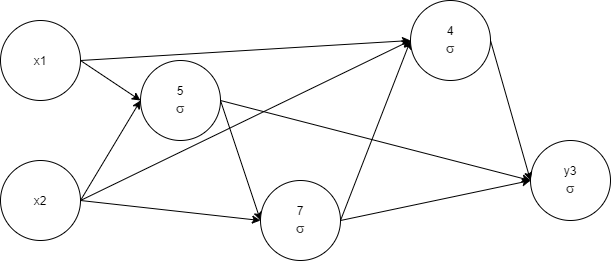
The network complexity was lowered, and as a result, training time was shortened too. We see the profit from the removal of network elements. Let's pay attention to the network complexity and start to measure it.
Introducing network complexity
Besides fitness, let's introduce another network metric - complexity. Our complexity function uses the amount of nodes and links in the network, together with weight and parameters difference from default values (1 is the simplest link weight - just transfer a signal, and 0 for default parameter - just absent value).
fn calculate_complexity(&mut self) {
let mut complexity = 0.0;
for _ in self.inputs.iter() {
complexity += 1.0;
}
for gene in self.genes.iter() {
complexity += 1.0;
for link in gene.inputs.iter() {
if link.weight != 1.0 {
complexity += 0.8;
} else {
complexity += 0.6;
}
}
let mut all_params_zero = true;
for p in &gene.params {
if *p != 0.0 {
all_params_zero = false;
break;
}
}
if !all_params_zero {
complexity += gene.params.len() as f32 * 0.4;
}
}
self.complexity = complexity;
}
From now, we can arrange individuals by fitness and complexity at the same time:
impl Ord for Individual {
fn cmp(&self, other: &Self) -> Ordering {
if self.fitness != other.fitness {
return
other.fitness.partial_cmp(&self.fitness).unwrap();
}
let a = self.genome.complexity;
let b = other.genome.complexity;
if a != b {
a.partial_cmp(&b).unwrap()
} else {
self.genome.len().cmp(&other.genome.len())
}
}
}
In this case, fitness is a priority, but as soon as two individuals get the same fitness, the least complex one becomes more important.
Evaluation result:
epochs=104, time=419.33ms, epochs/s=248.2, champion fitness=1,
complexity=15.200001, genes: 5, links: 10, species=21
x1, x2, 5 1 -< 1 0.81776786 -< 2 -1.0465963, 6 1 -< 5 1.2307372, 7
1 -0.04006207 -< 2 -0.16821101 -< 5 0.5667879, 4 1 -< 1 -0.9482097
-< 2 0.84273 -< 7 0.9627533, y3 1 -< 6 -< 4 1.1898354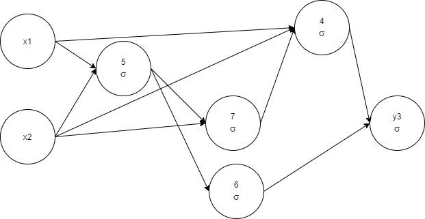
The training time reduced, which is expected since we choose fewer complex architectures. As you can note, the process is quite random, we got one more node compared to the previous run, just did it faster. The reason is our stop condition. If to continue evolution a little, there is a high chance to prune a node (see node 6 as a candidate).
Prune early
They're not always such a simple task, where reaching some fitness is an easy process. Evolving a network to reach the last few percent of fitness can take more time than all previous processes.
So in theory, I should start pruning early and operate with less complex architectures to reach the goal. Remember the "dropout_condition" function in the start environment - there we signal when to activate pruning mode, even when target fitness is not reached yet.
When the mode is switched on, we rise the weights of destructive mutations and lower weights of growing ones.
| Function | Probability | Probability in pruning mode |
|---|---|---|
| change link weight | 10 | 10 |
| slide link weight | 50 | 100 |
| add link | 10 | 10 |
| inject gene | 10 | 1 |
| toggle function | 10 | 1 |
| change parameters | 10 | 1 |
| unlink | 10 | 100 |
| remove gene | 10 | 10 |
epochs=117, time=396.83ms, epochs/s=295.5, champion
fitness=0.9999994, complexity=8, genes: 2, links: 5, species=6
x1, x2, 4 1 -< 1 1.2193546 -< 2 -1.4424781, y3 1 -< 1 -1.0417894 -<
2 1.023965 -< 4 1.6750889

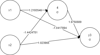
Again, as more priority is given to less complex networks, the training took less time. And for sure, the final network will perform faster as it is less complex.
When pruning can be avoided
The above evaluation was done with all nodes as neurons just to demonstrate the algorithm. But remember, our genetic algorithm can use any node function. It makes sense to give the algorithm more options to select. From now, nodes can use one of the functions below:
- σ (Leaky ReLU), the neuron node
- Σ (sum)
- ⩒ (XOR)
Let see what will be selected to build the final network:
epochs=21, time=89.80ms, epochs/s=236.0, champion fitness=1,
complexity=4.2, genes: 1, links: 2, species=3
x1, x2, y3 3 -< 1 -< 2

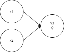
Ideally, it’s absolutely enough to use just one XOR node to solve the XOR classification problem.
Conclusion
The genetic algorithm is known for its ability to create effective network architectures. With a simple addition of measuring the complexity of the network, this algorithm can also create an efficient pruning strategy.
The above chapters demonstrated basic steps to automate pruning with GA and as a consequence to improve model performance. For sure, there are places to improve the algorithm, but it is quite reliable even in the basic form.


